Creating some rarefaction curves for butteryfly data
data(warande) # example data included in package
dplyr::glimpse(warande)
#> Rows: 2,976
#> Columns: 5
#> $ date         <date> 2009-06-19, 2009-07-01, 2009-08-13, 2009-08-30, 2010-06-…
#> $ species_name <chr> "Bruine huismot", "Oranje iepentakvlinder", "Oranje worte…
#> $ year         <dbl> 2009, 2009, 2009, 2009, 2010, 2010, 2010, 2010, 2010, 201…
#> $ number       <dbl> 1, 1, 1, 1, 1, 1, 1, 1, 1, 1, 1, 1, 1, 1, 1, 1, 1, 1, 1, …
#> $ MicroMacro   <chr> "Micro", "Macro", "Macro", "Macro", "Macro", "Macro", "Ma…
Incidence based rarefaction curve
Splitting it up in Micro and Macro
Getting the data in the right shape
iNEXT expects incidence data to consist of a list of frequencies, with the first element of the list the number of sampling units, followed by the incidence frequencies. The length of the list should be the number of observed species minus one.
This package provides a function to convert a dataframe with a known shape (and exactly this shape) to this format.
You can provide a column that will be used to split your dataframe into assemblages.
Let’s set our assemblage to MicroMacro, so have one assembly for the Micro butterflies, and one for the Macro butterflies.
rare_out_inc <-
  iNEXT::iNEXT(
    convert_to_incidence_freq(warande, assemblage = MicroMacro),
    datatype = "incidence_freq",
    nboot = 50 # you might want to set this a bit higher
    )

rare_out_inc
#> Compare 2 assemblages with Hill number order q = 0.
#> $class: iNEXT
#>
#> $DataInfo: basic data information
#>   Assemblage   T    U S.obs     SC Q1 Q2 Q3 Q4 Q5 Q6 Q7 Q8 Q9 Q10
#> 1      Macro 162 2230   312 0.9680 72 43 27 19 24 16  9 14  4  13
#> 2      Micro 149  746   203 0.8921 81 38 30 12  5  6  5  3  1   4
#>
#> $iNextEst: diversity estimates with rarefied and extrapolated samples.
#> $size_based (LCL and UCL are obtained for fixed size.)
#>
#>    Assemblage   t        Method Order.q         qD     qD.LCL     qD.UCL
#> 1       Macro   1   Rarefaction       0  13.765432  13.197970  14.332895
#> 10      Macro  81   Rarefaction       0 259.802910 251.861150 267.744671
#> 20      Macro 162      Observed       0 312.000000 298.979487 325.020513
#> 30      Macro 239 Extrapolation       0 337.999160 319.467414 356.530907
#> 40      Macro 324 Extrapolation       0 353.816856 329.290932 378.342781
#> 41      Micro   1   Rarefaction       0   5.006711   4.615889   5.397534
#> 50      Micro  74   Rarefaction       0 147.884654 138.347199 157.422109
#> 60      Micro 149      Observed       0 203.000000 188.896261 217.103739
#> 70      Micro 220 Extrapolation       0 234.001881 215.712868 252.290894
#> 80      Micro 298 Extrapolation       0 255.307935 232.128701 278.487170
#>            SC     SC.LCL     SC.UCL
#> 1  0.09081692 0.08504943 0.09658442
#> 10 0.93026235 0.92382346 0.93670123
#> 20 0.96795077 0.96123655 0.97466500
#> 30 0.98185989 0.97485443 0.98886535
#> 40 0.99032209 0.98459226 0.99605192
#> 41 0.05474241 0.04716427 0.06232055
#> 50 0.79818804 0.77706973 0.81930635
#> 60 0.89210493 0.87279388 0.91141598
#> 70 0.93111330 0.91215329 0.95007330
#> 80 0.95792181 0.94150576 0.97433786
#>
#> NOTE: The above output only shows five estimates for each assemblage; call iNEXT.object$iNextEst$size_based to view complete output.
#>
#> $coverage_based (LCL and UCL are obtained for fixed coverage; interval length is wider due to varying size in bootstraps.)
#>
#>    Assemblage         SC   t        Method Order.q         qD     qD.LCL
#> 1       Macro 0.09081810   1   Rarefaction       0  13.765607  13.201546
#> 10      Macro 0.93026235  81   Rarefaction       0 259.802915 247.878558
#> 20      Macro 0.96795077 162      Observed       0 312.000000 290.971001
#> 30      Macro 0.98185989 239 Extrapolation       0 337.999160 309.959368
#> 40      Macro 0.99032209 324 Extrapolation       0 353.816856 320.697469
#> 41      Micro 0.05474241   1   Rarefaction       0   5.006711   4.599338
#> 50      Micro 0.79818804  74   Rarefaction       0 147.884652 133.395165
#> 60      Micro 0.89210493 149      Observed       0 203.000000 180.158429
#> 70      Micro 0.93111330 220 Extrapolation       0 234.001881 205.719840
#> 80      Micro 0.95792181 298 Extrapolation       0 255.307935 222.683841
#>        qD.UCL
#> 1   14.329668
#> 10 271.727272
#> 20 333.028999
#> 30 366.038953
#> 40 386.936244
#> 41   5.414084
#> 50 162.374138
#> 60 225.841571
#> 70 262.283922
#> 80 287.932030
#>
#> NOTE: The above output only shows five estimates for each assemblage; call iNEXT.object$iNextEst$coverage_based to view complete output.
#>
#> $AsyEst: asymptotic diversity estimates along with related statistics.
#>   Assemblage         Diversity  Observed Estimator      s.e.      LCL      UCL
#> 1      Macro  Species richness 312.00000 371.90698 16.735917 339.1052 404.7088
#> 2      Macro Shannon diversity 193.08584 210.89968  4.001470 203.0569 218.7424
#> 3      Macro Simpson diversity 142.75175 151.57339  3.954126 143.8234 159.3233
#> 4      Micro  Species richness 203.00000 288.74956 19.971133 249.6069 327.8923
#> 5      Micro Shannon diversity 123.68027 152.96329  6.798172 139.6391 166.2875
#> 6      Micro Simpson diversity  81.96112  91.45944  5.793695  80.1040 102.8149
And plot it:
iNEXT::ggiNEXT(rare_out_inc)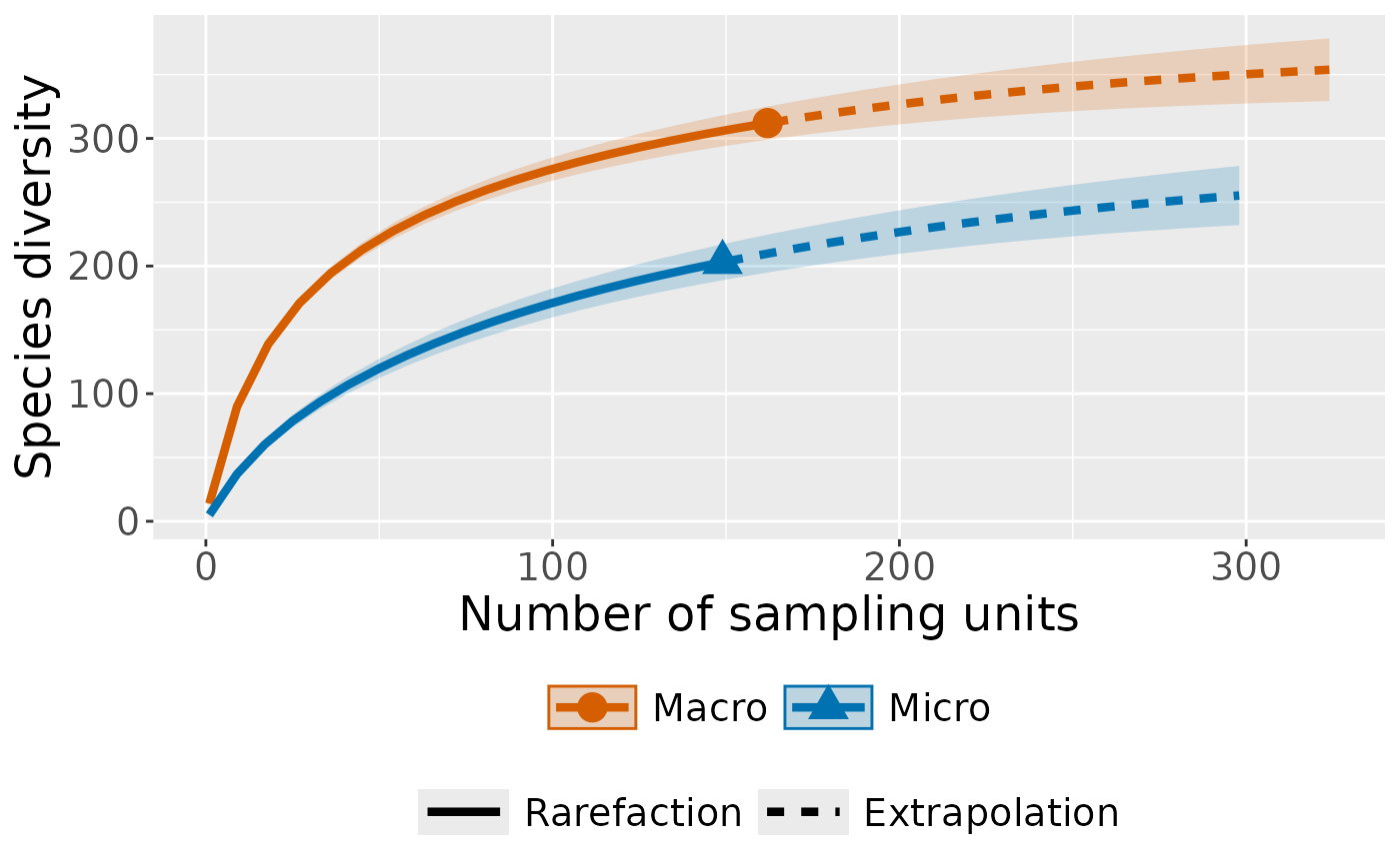
Abundance based
Splitting it up in Micro and Macro
Getting the data in the right shape
Plug this into iNEXT:
rare_out_abun <-
iNEXT::iNEXT(convert_to_abundance(warande, assemblage = MicroMacro),
datatype = "abundance",
nboot = 50 # you might want to set this a bit higher
)
rare_out_abun
#> Compare 2 assemblages with Hill number order q = 0.
#> $class: iNEXT
#>
#> $DataInfo: basic data information
#> Assemblage n S.obs SC f1 f2 f3 f4 f5 f6 f7 f8 f9 f10
#> 1 Macro 3764 312 0.9822 67 38 29 19 22 14 12 9 3 9
#> 2 Micro 1212 203 0.9349 79 39 28 11 6 4 4 3 4 2
#>
#> $iNextEst: diversity estimates with rarefied and extrapolated samples.
#> $size_based (LCL and UCL are obtained for fixed size.)
#>
#> Assemblage m Method Order.q qD qD.LCL qD.UCL SC
#> 1 Macro 1 Rarefaction 0 1.0000 1.0000 1.0000 0.01518561
#> 10 Macro 1882 Rarefaction 0 263.1436 253.8563 272.4309 0.96069585
#> 20 Macro 3764 Observed 0 312.0000 299.0934 324.9066 0.98220515
#> 30 Macro 5547 Extrapolation 0 336.5489 318.9805 354.1172 0.98960299
#> 40 Macro 7528 Extrapolation 0 352.0598 328.3744 375.7452 0.99427725
#> 41 Micro 1 Rarefaction 0 1.0000 1.0000 1.0000 0.06690595
#> 50 Micro 606 Rarefaction 0 149.2826 140.7580 157.8073 0.87805769
#> 60 Micro 1212 Observed 0 203.0000 188.6808 217.3192 0.93487158
#> 70 Micro 1786 Extrapolation 0 232.8697 213.1493 252.5901 0.95920486
#> 80 Micro 2424 Extrapolation 0 253.1737 227.1766 279.1707 0.97574539
#> SC.LCL SC.UCL
#> 1 0.01401061 0.01636062
#> 10 0.95735174 0.96403996
#> 20 0.97859523 0.98581507
#> 30 0.98541915 0.99378684
#> 40 0.99072191 0.99783258
#> 41 0.05695751 0.07685438
#> 50 0.86533741 0.89077798
#> 60 0.92185533 0.94788784
#> 70 0.94546342 0.97294629
#> 80 0.96349177 0.98799902
#>
#> NOTE: The above output only shows five estimates for each assemblage; call iNEXT.object$iNextEst$size_based to view complete output.
#>
#> $coverage_based (LCL and UCL are obtained for fixed coverage; interval length is wider due to varying size in bootstraps.)
#>
#> Assemblage SC m Method Order.q qD qD.LCL
#> 1 Macro 0.01518581 1 Rarefaction 0 1.000013 0.9667868
#> 10 Macro 0.96069585 1882 Rarefaction 0 263.143565 249.7041435
#> 20 Macro 0.98220515 3764 Observed 0 312.000000 291.4637490
#> 30 Macro 0.98960299 5547 Extrapolation 0 336.548863 308.4736916
#> 40 Macro 0.99427725 7528 Extrapolation 0 352.059815 318.4303637
#> 41 Micro 0.06690595 1 Rarefaction 0 1.000000 0.9173293
#> 50 Micro 0.87805770 606 Rarefaction 0 149.282641 133.0267913
#> 60 Micro 0.93487158 1212 Observed 0 203.000000 177.3717340
#> 70 Micro 0.95920486 1786 Extrapolation 0 232.869717 200.2388336
#> 80 Micro 0.97574539 2424 Extrapolation 0 253.173653 214.6256516
#> qD.UCL
#> 1 1.033240
#> 10 276.582987
#> 20 332.536251
#> 30 364.624035
#> 40 385.689267
#> 41 1.082671
#> 50 165.538491
#> 60 228.628266
#> 70 265.500601
#> 80 291.721655
#>
#> NOTE: The above output only shows five estimates for each assemblage; call iNEXT.object$iNextEst$coverage_based to view complete output.
#>
#> $AsyEst: asymptotic diversity estimates along with related statistics.
#> Assemblage Diversity Observed Estimator s.e. LCL
#> 1 Macro Species richness 312.00000 371.05010 16.483480 338.74307
#> 2 Macro Shannon diversity 131.17683 138.38326 3.099284 132.30877
#> 3 Macro Simpson diversity 64.73642 65.85180 2.670176 60.61835
#> 4 Micro Species richness 203.00000 282.94680 21.367817 241.06665
#> 5 Micro Shannon diversity 57.86578 65.89988 3.420808 59.19521
#> 6 Micro Simpson diversity 14.77632 14.94635 1.263246 12.47044
#> UCL
#> 1 403.35712
#> 2 144.45774
#> 3 71.08525
#> 4 324.82695
#> 5 72.60454
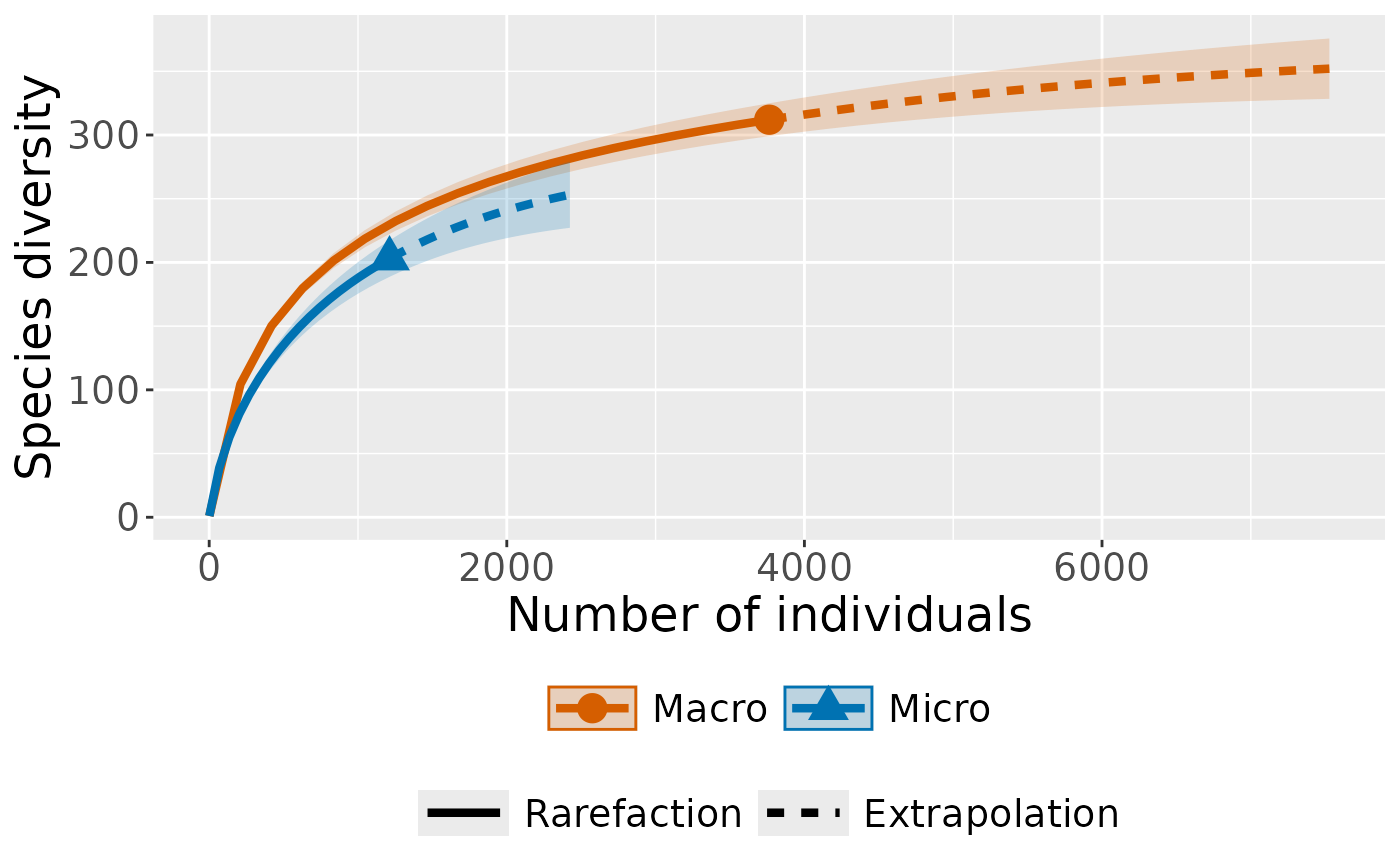
#> 6 17.42227And plot it:
iNEXT::ggiNEXT(rare_out_abun)